Note: Input and output files could be found here.

Contents

• 1. Input
• 2. Output
• 3. Improve accuracy with scaling factor
• 4. Add more references in GaussView
• 5. Apply scaling factor with py.NMR

1. Input

An example of NMR calculation for benzene in d-chloroform will be discussed in this post. The geometry of benzene was optimized at B3LYP/6-311+G(2d,p) level of theory in gas phase. The input file for optimization is attached following:

%nprocshared=8
%mem=10GB
#p opt rb3lyp/6-311+g(2d,p)

Benzene//optimization

0 1
 C                  0.12565445    0.25654450    0.00000000
 C                  1.52081445    0.25654450    0.00000000
 C                  2.21835245    1.46429550    0.00000000
 C                  1.52069845    2.67280450   -0.00119900
 C                  0.12587345    2.67272650   -0.00167800
 C                 -0.57172755    1.46452050   -0.00068200
 H                 -0.42410455   -0.69577250    0.00045000
 H                  2.07032245   -0.69596850    0.00131500
 H                  3.31803245    1.46437550    0.00063400
 H                  2.07089845    3.62494750   -0.00125800
 H                 -0.42424855    3.62500750   -0.00263100
 H                 -1.67133155    1.46470350   -0.00086200

The optimized geometry is used for NMR (NMR=GIAO) calculation at B3LYP/6-311+G(2d,p) level of theory with SMD solvation model of chloroform.

%nprocshared=8
%mem=10GB
#p nmr=giao rb3lyp/6-311+g(2d,p) scrf=(smd,solvent=chloroform)

Benzene//NMR

0 1
 C                 -0.01990700   -1.39174700    0.00000100
 C                  1.19536900   -0.71306400   -0.00000700
 C                  1.21525700    0.67862700    0.00001100
 C                  0.01984500    1.39174800   -0.00000100
 C                 -1.19533800    0.71311600   -0.00000800
 C                 -1.21522700   -0.67868000    0.00000600
 H                 -0.03531700   -2.47537300   -0.00000600
 H                  2.12604500   -1.26833800   -0.00000900
 H                  2.16140200    1.20710800   -0.00000200
 H                  0.03539700    2.47537200    0.00000200
 H                 -2.12608400    1.26827300   -0.00001000
 H                 -2.16144000   -1.20704000    0.00001600

2. Output

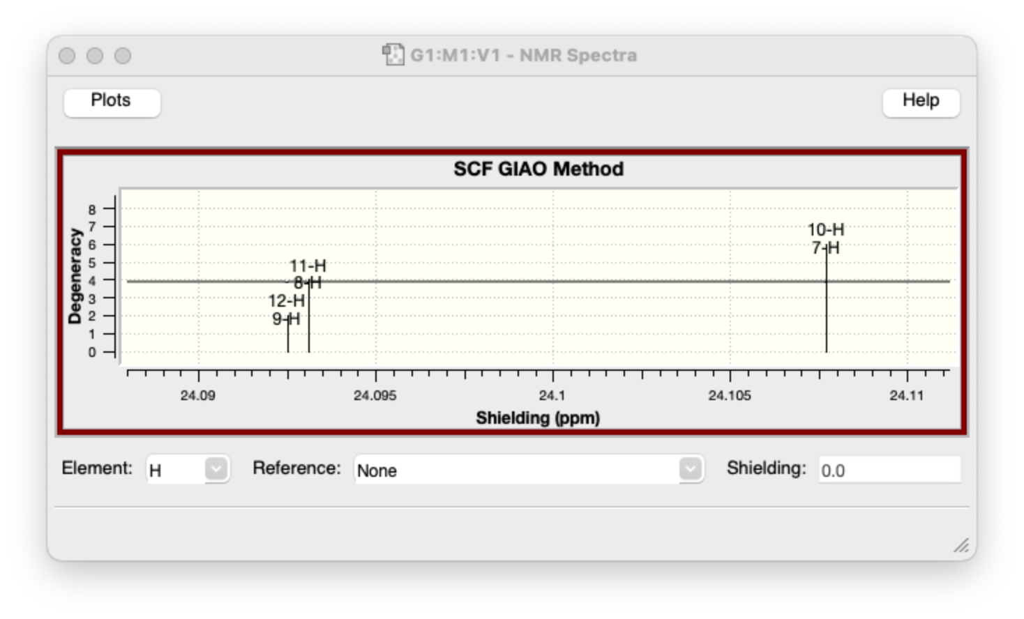
Open the output file with GaussView, go to “Results -> NMR”, choose “H” from “element”, we could get the magnetic shielding tensors σ (in ppm).

You could also use “Reference” like TMS, to get the chemical shift δ, to compare with experimental data.

In this demo calculation, the computed shielding tensors σ for all protons are 24.0925, 24.0931 and 24.1077 ppm, the chemical shift δ are 7.7896, 7.7890 and 7.7744. The experimental chemica shift of benzene in d-chloroform is 7.36.

3. Improve accuracy with scaling factor

Empirical scaling technique could improve the accuracy using scaling factors. CHESHIRE is a website with a lot of scaling factors at different calculation levels. Visit this website and go to “Scaling factor”, we could find this:

Table #1b: 1H and 13C scaling factors for 14 Chloroform DFT and Wavefunction methods (G09 - SMD solvation model)

Geometry (opt&freq): B3LYP/6-311+G(2d,p) (gas phase)
NMR (nmr=method): B3LYP/6-311+G(2d,p) (giao, scrf)

is exactly what we want. We need the slope = -1.0781 and intercept = 31.9786, and we could calculate the scaled chemical shift δ_scaled with following equation:

• δ_scaled (ppm): Chemical shift after applied with scaling factor
• slope and intercept: Scaling factors from CHESHIRE
• σ (ppm): Computed magnetic shielding tensors from Gaussian output

So, the scaled chemical shift δ_scaled in this demo calculation are 7.3148, 7.3143 and 7.3007, much closer to the experimental value than those before scaling.

4. Add more references in GaussView

1. Open the GaussView dictionary, open the nmr.data in data folder with text edit. For macOS users, the nmr.data locates at /Applications/gv/data/nmr.data.
2. Add the references at the end of file, for example: H 32.3685 “TMS wB97XD/6-31+G(d,p) GIAO”
3. Re-open GaussView, you could find the new reference in NMR window.

5. Apply scaling factor with py.NMR

py.NMR is end of support. The basic functionalities have been combined into py.Aroma, a multi-functional tool for aromaticity analyses. Please check the homepage of py.Aroma for more information.

py.NMR is a Python program for applying scaling factors to computed shielding tensors. The latest version of py.NMR could be freely download from GitHub.

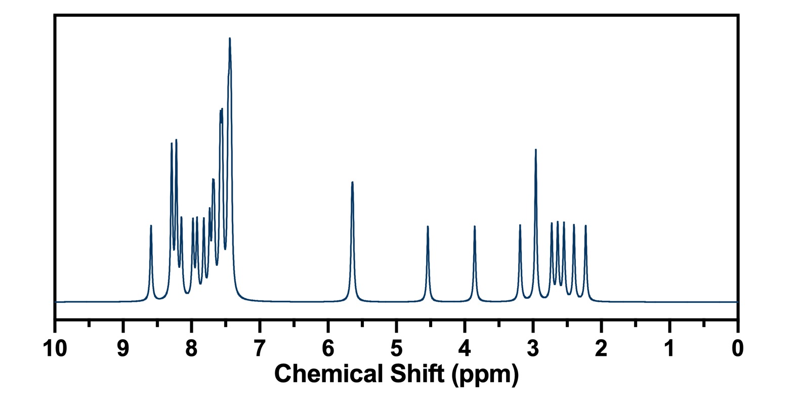
In py.NMR, Lorentzian function for line broadening will be applied to the scaled chemical shift, and the sprctrum data would be saved in an Excel .xlsx file at the same dictionary as the Gaussian output.

Users can plot the scaled NMR spectrum with the data points in Excel file. More detail about usage of py.NMR, please refer to the user manual on GitHub.