This blog is part of theme collection: Visualization of Aromaticity, see post of AICD in this collection.

1 Background

Gauge-including magnetically induced currents (GIMIC) is a useful tool for aromaticity analyses. In this blog, I will show you how to do the GIMIC calculation and visualize the results using ParaView.

Different to AICD, GIMIC can use GIAO method for NMR calculation, this may be better than CSGT. But, GIMIC does not support to decompose the contribution from different orbitals.

2 Procedure

The procedure of conducting GIMIC calculation will be discussed in this section. All calculation files could be found from here.

2.1 NMR Calculations

NMR calculations by Gaussian are necessary before GIMIC analyses. Input files for open-shell and close-shell calculation are different:

Closed-shell system

%chk=methylazulene_GIMIC.chk
# nmr=giao rb3lyp/6-31g(d) iop(10/33=2) int=nobasistransform

Title

Geometry specification

Open-shell system

%chk=methylazulene_GIMIC.chk
# nmr=giao ub3lyp/6-31g(d) iop(10/33=2) int=nobasistransform gfprint pop=full

Title

Geometry specification

2.2 Generate XDENS & MOL Files

XDENS and MOL files are necessary for GIMIC analyses. After finishing the NMR calculations, copy the .fchk (for closed-shell calculations) or .log (for open-shell calculations) to the computer with GIMIC installed.

Copy the BasisSet.py and Gaussian2gimic.py files in the ~/gimic/tools/g092gimic folder to the same dictionary with .fchk or .log file. Execute following command:

(for closed-shell) ./Gaussian2gimic.py --input=filename.fchk
(for open-shell) ./Gaussian2gimic.py --input=filename.log

The XDENS and MOL files would be generated in the same dictionary.

2.3 GIMIC Calculation

An example of GIMIC input file is shown in following.

calc=cdens
basis="./MOL"
xdens="./XDENS"
openshell=false 
magnet=[0,0,1]

Grid(base) { 
    type=even
    origin=[-8.0, -7.0, -6.0]
    ivec=[1.0, 0.0, 0.0]
    jvec=[0.0, 1.0, 0.0]
    lengths=[16.0, 14.0, 12.0]
    grid_points=[50, 50, 50]
}

Advanced {
    spherical=off
    diamag=on
    paramag=on
}

Essential {
    acid=on
    jmod=on
}

Here are some important keyword:

• openshell: For open-shell species, set it to true.
• magnet: Direction of external magnetic field, similar to the -b command in AICD.
• origin: Origin of grid, from bottom left cornor.
• lengths: Size of grid.
• grid_points: Number of grid points in each axis.

More details about the input file, please refer to the user manual.

Save the input file in the same folder with XDENS and MOL files, and name it as gimic.inp, then, execute gimic command, the GIMIC calculation would run in seconds.

2.4 Visualization

After several minutes, some new files would be generated after finishing the calculation. To visualize the results, we will use ParaView (free download from homepage). In order for ParaView to display the molecular structure correctly, the .cml format file of the molecule also needs to be generated before visualization. Here are two method to convert the .xyz into .cml.

1. Use OpenBabel, Windows user can download from homepage of OpenBabel. In my experience, it does not work normally on Mac computer. Please note that, you also need to convert the unit from Angstrom to Bohr, since .vti file generated by GIMIC use Bohr unit.

2. Use xyz2cml, it can convert mol.xyz in the current dictionary into mol-bohr.cml, which also convert the unit from Angstrom to Bohr.

GIMIC and ParaView can do a lot, in this section I will only present how to draw the stream line of ring current. Here is the general procedure.

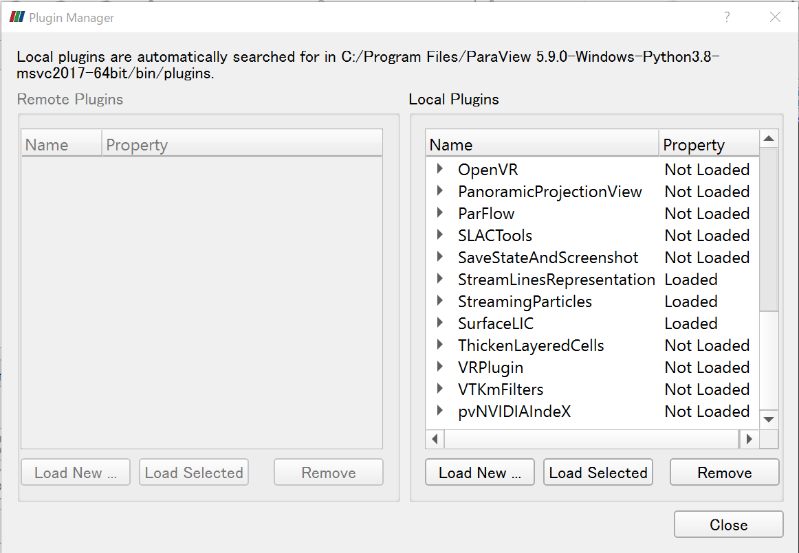
1) Open ParaView, load plugins from Tools -> Manage Plugins, select the StreamLinesRepresentation, StreamingParticles and SurfaceLIC, and click Load Selected.

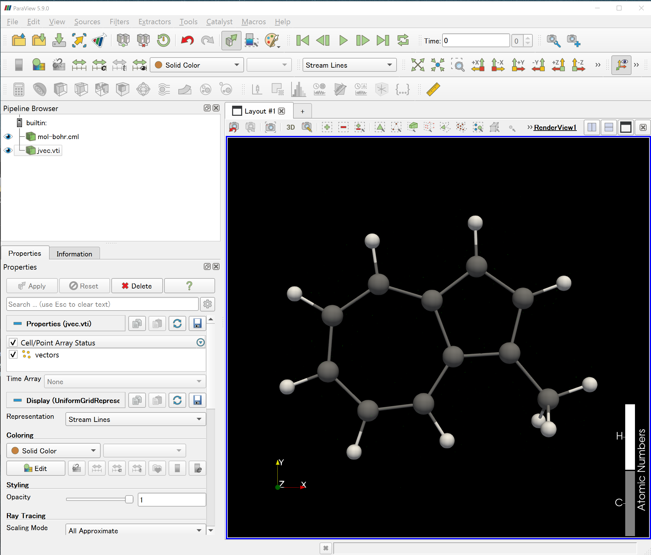
2) Load mol-bohr.cml and jvec.vti files to the ParaView.

3) Choose Streame Lines in the Representation.

4) Set the coloring, step length, number of particles and max time to a proper value until you could see the ring current stream lines in the main window.

2.5 Export movie

ParaView has the built-in function to export movie, but it does not work on my computer. My solution is, save .png images, and combine them into a movie.

1) Choose View -> Animation View, enlarge the number of frames (for example, 10000).

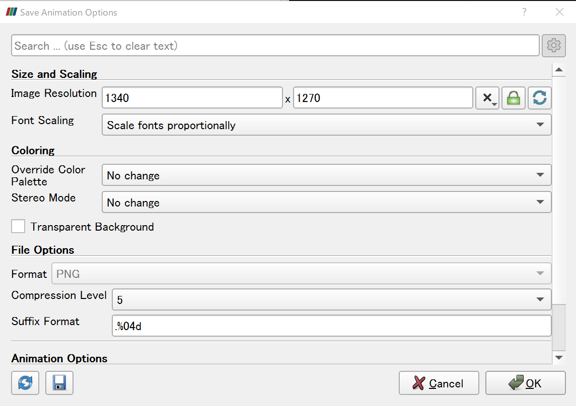
2) Click File -> Save Animation, and save the .png files.

3) I use ffmpeg program to convert the .png images into .mp4 movie. The command is:

ffmpeg -framerate 30 -i image_%03d.png -vcodec libx264 -pix_fmt yuv420p -r 60 out.mp4

By this command, 10000 images would be saved as a about 33 second mp4 movie.