Visualization of Aromaticity: AICD
This blog is part of theme collection: Visualization of Aromaticity, see post of GIMIC in this collection.
1. Background
Anisotropy of the Induced Current Density (AICD) has been widely used for aromaticity analyses. More basic knowledge about AICD, please refer to this review paper. In this blog, I will show you how to make the AICD plot and apply AICD to your research. AICD is a free and open source program, you can obtain the program freely from the author (E-mail to Dr.Herges: rherges@oc.uni-kiel.de).
The biggest feature of AICD is that it can separate the orbital contribution (from all molecular orbitals, or from π orbitals only), this is useful when analyze the aromaticity from the contribution of π electrons.
2. Install AICD on a Linux machine
This is a guide for install AICD 3.0.4, if you are using different version, this procedure may be not work.
(1) Run following command in termial window.
tar xvf AICD-3.0.4.tbz
cd AICD-3.0.4
make
(2) Add following environment variable to the ~/.bashrc file:
alias AICD=~/path_to/AICD-3.0.4/AICD
(3) Add permision to the AICD program:
chmod +x ~/path_to/AICD-3.0.4/* -R
(4) Install povchem 1.0: Download povchem.c, and run following command:
cc povchem.c -o povchem -lm
(5) Add following environment variable to the ~/.bashrc file:
alias povchem=~/path_to/pocvhem
(6) Copy povchem.cfg and periodic.tab files to /AICD-3.0.4/povchem. Maybe you need to modify the /AICD-3.0.4/AICD file using texteditor, the row No.404, replace the povchem to the full path of povchem.
(7) Install PovRay: Download PovRay from homepage, and run following command:
tar -xvf povlinux-3.6.tar
cd povlinux-3.6
./install -no-arch-check
(9) Run AICD in terminal window, if you could see following message, the program was installed successfully on the computer.
Zweck: Extraktion der induzierten Stromdichte (ICD)
       aus einem oder mehreren Gaussian98-log-files.

Dieses Script liest die angegebenen Dateien und
wandelt sie in mehrere Dateien um.

Aufruf: /home/hpc/wang/AICD-3.0.4/AICD  Gaussian98-output-file(s)
3. Procedure
In this section, I will use an example of 1-methylazulene as a demo calculation to explain how to make the AICD plot. Calculation files could be download from here. I also uploaded a slide for AICD analysis of cyclo[18]carbon, it is also a good example for AICD analysis.
3.1 NMR calculation
Before doing this NMR calculation, make sure you have already optimized your geometry. The 1-methylazulene was optimized at ωB97X-D/6-31G(d) level of theory. The input file for NMR calculation have to contain following keywords:
Contribution from all orbitals
# nmr=csgt b3lyp/6-31g(d) iop(10/93=1)

 title

 0 1
 […Coordinates…]

 filename.txt
Contribution from specified orbitals
# nmr=csgt b3lyp/6-31g(d) iop(10/93=2)

title

0 1
[…Coordinates…]

filename.txt

orbital number 1
orbital number 2
...
There are several important points for the input file:
- Use
CSGTmethod for NMR calculation. - B3LYP/6-31G(d) is often enough to yield qualitatively satisfactory result.
- Include the
IOp(10/93=n)keywords: n = 1 for calculating contribution from all orbitals and n = 2 for calculating contribution from specified orbitals. - A .txt file including ring current grid information would be saved during the NMR calculation, so, you need to specify a file name for it.
- Include the molecular orbital numbers (those will be considered for NMR calculation) in the end of input file if you use
IOp(10/93=2). (For unrestricted calculation, alpha orbitals and beta orbitals are separated, the orbital numbers of alpha orbital are same as those displayed in GaussView, but, the orbital numbers of beta orbitals are those in GaussView plus occupied orbital numbers. e.g., for the ith alpha and beta orbitals, and total n occupied orbitals, you need to write “i” and “i+n”.)

Submit this input file to Gaussian calculation. Once the calculation is completed, .log (or .out) and .txt files would be generated, these 2 files are necessary for next step AICD calculation.
3.2 AICD calculation
Execute following command for AICD calculation:
AICD option1 value1 option2 value2 --povrayinput -c xxx.log
There are some useful option for make high quality AICD plots:
-m n
Molecular view in AICD plots, n = 1-4. (1: single view, surface only; 2: single view, surface and arrows; 3: multi view, surface only; 4: multi view, surface and arrows)

-b x y z
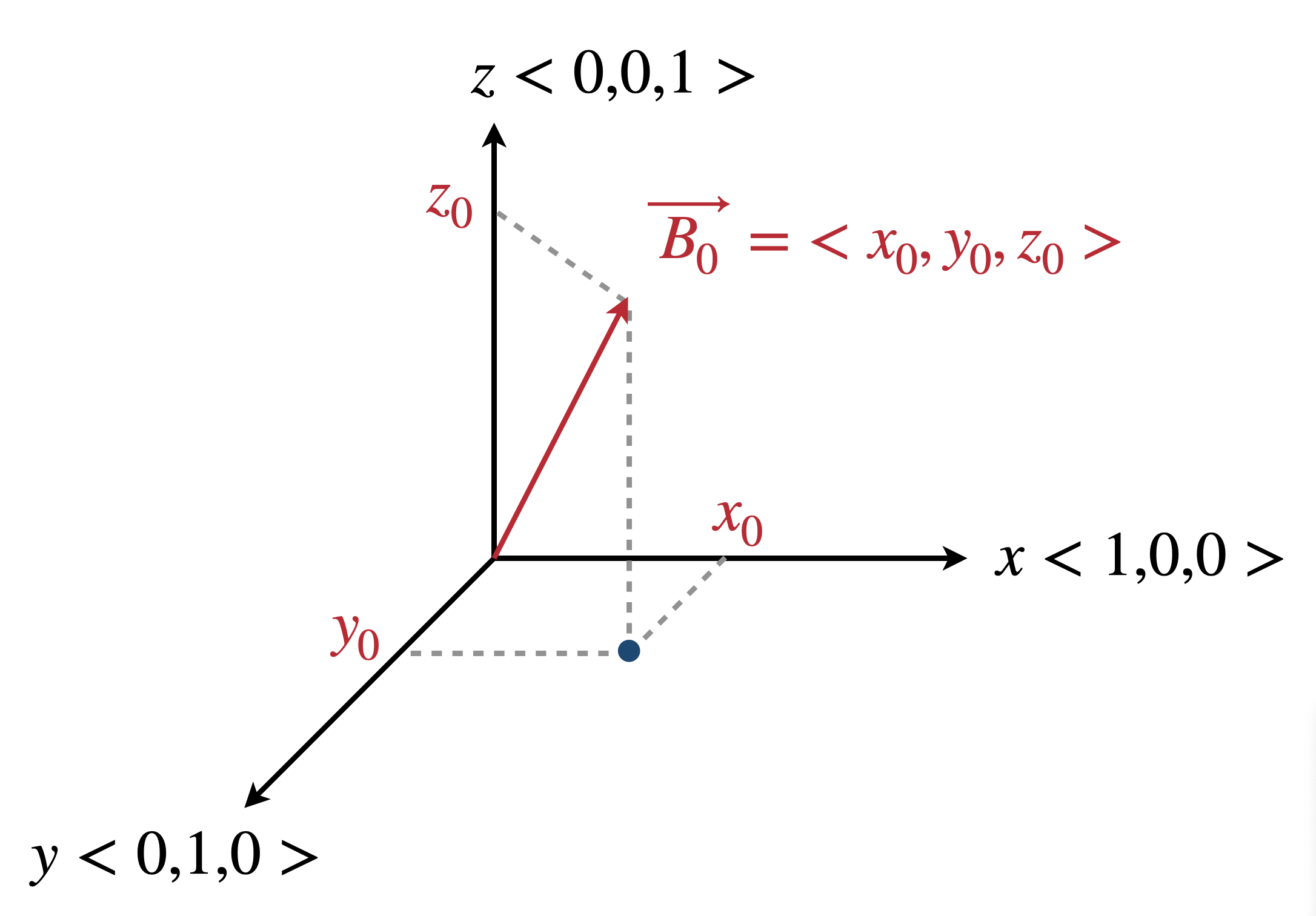
Direction of external magnetic field (default is 0 0 1), the external magnetic field is defined in vector space with x, y, z direction. The external is only defined in direction, the magnitude is out of consideration (e.g.: 0 0 1 is same as 0 0 2).
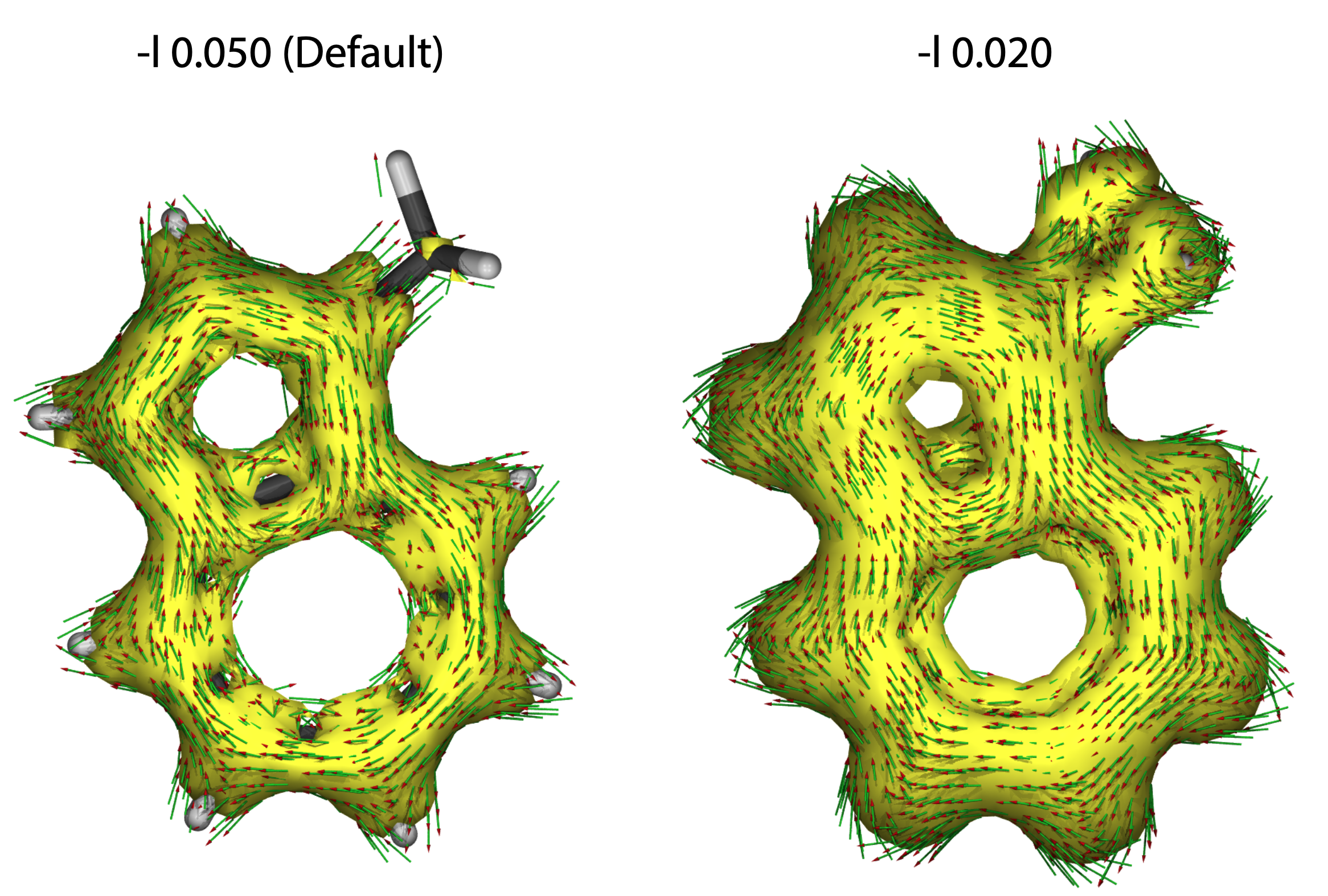
-l r
Iso-surface value.
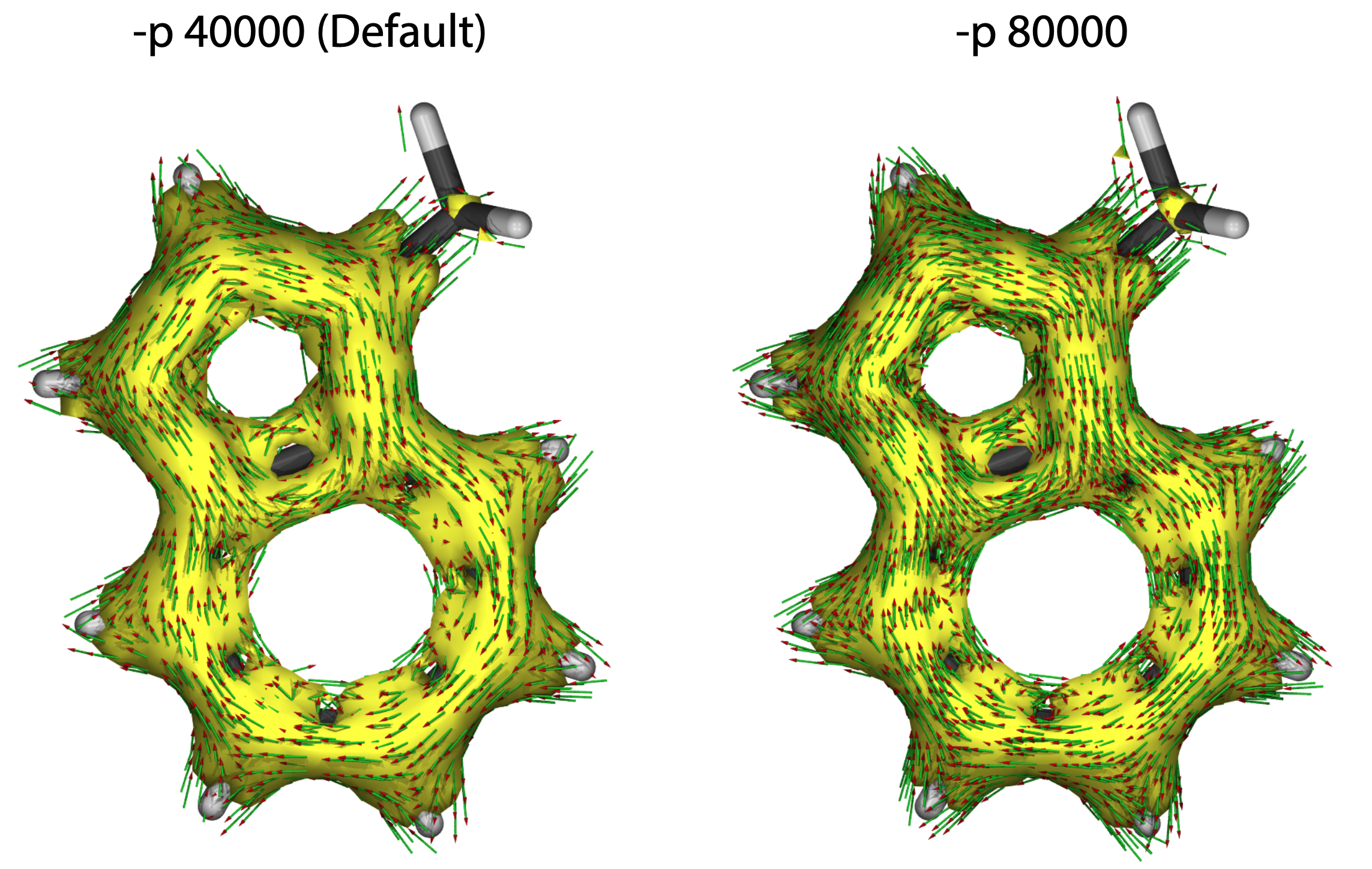
-p n
Number of data points, default is 40000, larger n value will generate more arrows and smoother iso-surface. More computational cost is needed.
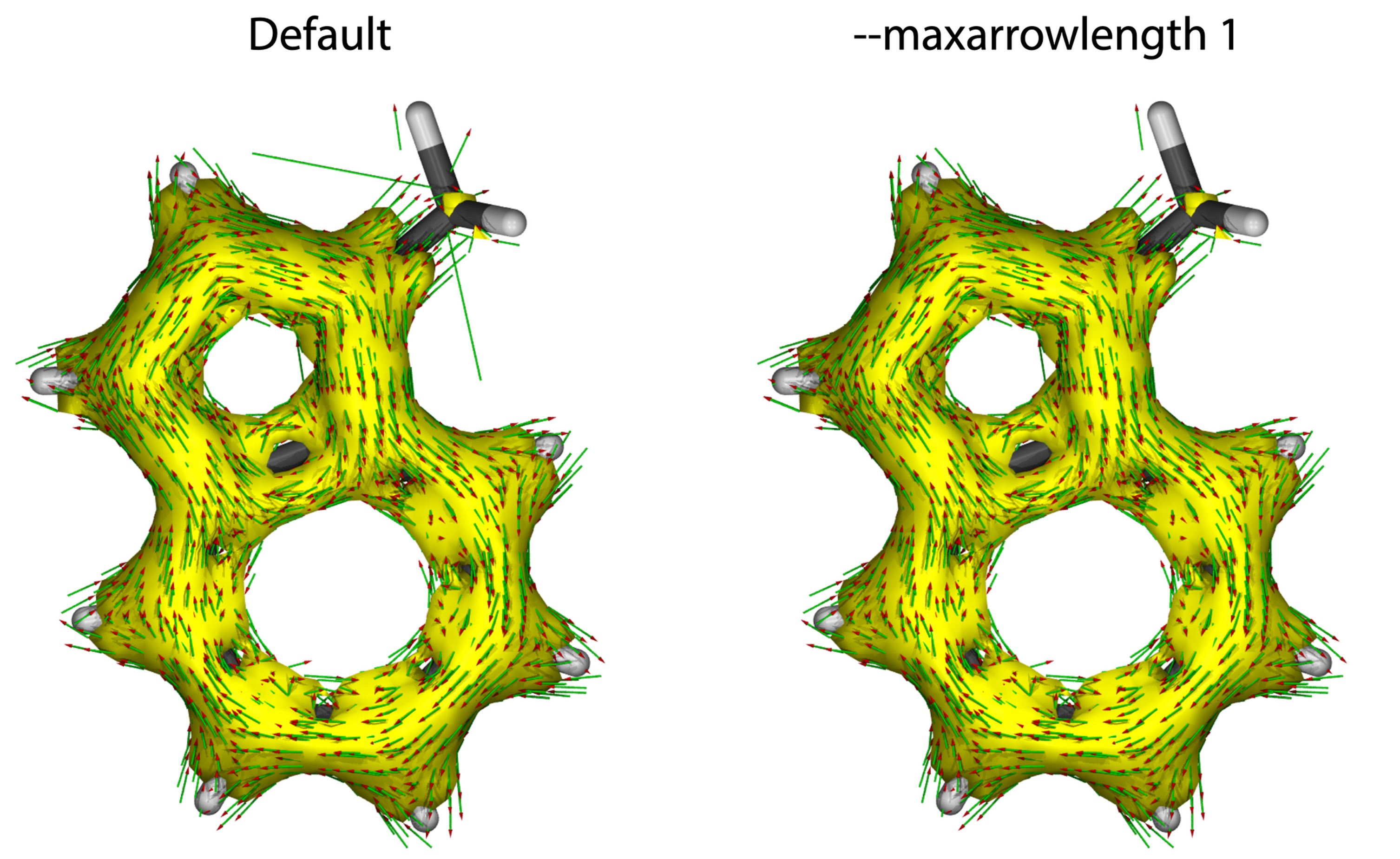
--maxarrowlength f
Define the maximum of arrow length, the arrows longer than value f would not be displayed in AICD map (similar option: --minarrowlength)
-s
Smoothly graphical representation, needs more computational cost.
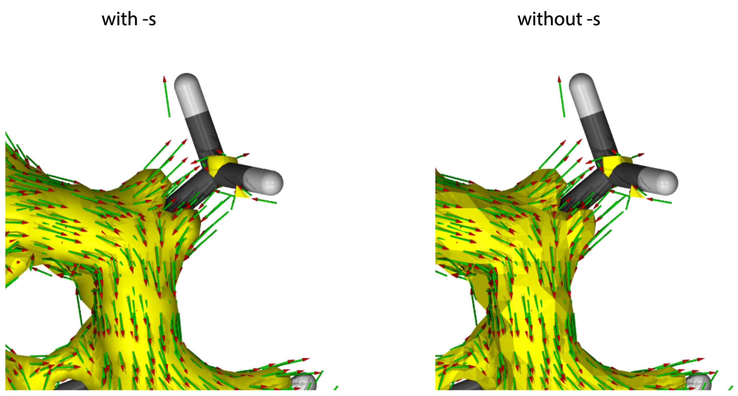
More options can be found from AICD -h command. After AICD calculation, several files would be generated and we need the files in the folder named as “xxxxxxxxxxxxxx.d”. Copy this folder to a computer with POV-Ray installed.
3.3 AICD visualization
To visualize the AICD plot, image rendering software, POV-Ray, is needed. POV-Ray could be freely download from the homepage. Open the “RenderMich.pov” file with POV-Ray in the “xxxxxxxxxxxxxx.d” folder. Choose the resolution and click “Run” icon. The AICD plot will be shown in a new window, and it will be saved as .png image at current path automatically, so, you don’t need to save it manually.
Here are some common issues when using the POV-Ray:
(1) Molecular structure could not be fully displayed
The following figure shows how the POV-Ray renders an image:
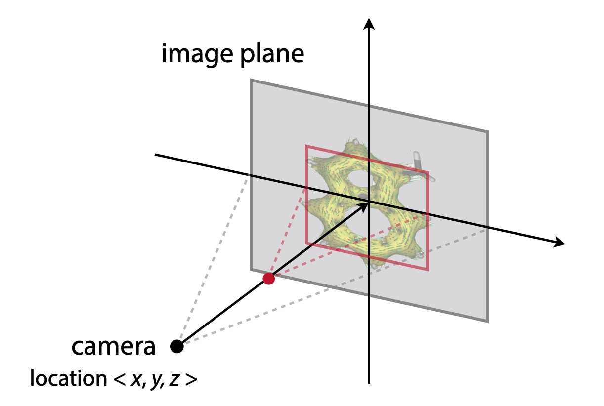
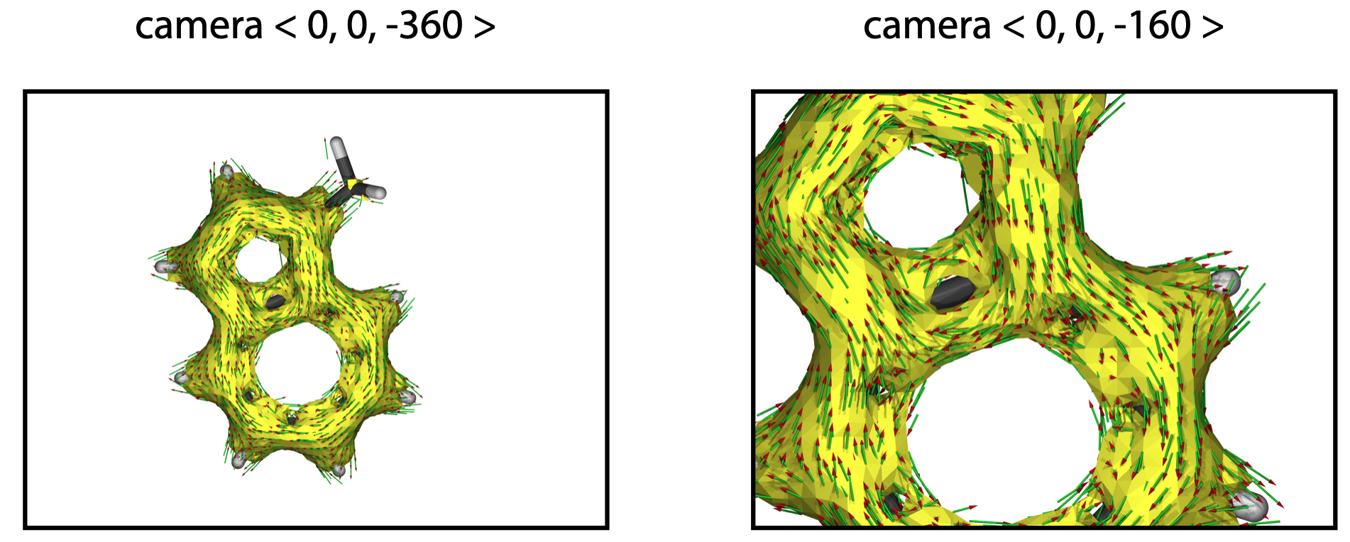
If the molecule is not displayed in full, please modify the camera - location coordinate <x, y, z> in the “RenderMich.pov” file. More negative z value will give smaller size molecule.
camera{
  location <  0, 0, -160 >
  direction < 0, 0, 2 >
  sky < 0, 1, 0 >
  up < 0, 1, 0 >
  right < 1.333, 0, 0 >
  orthographic
}
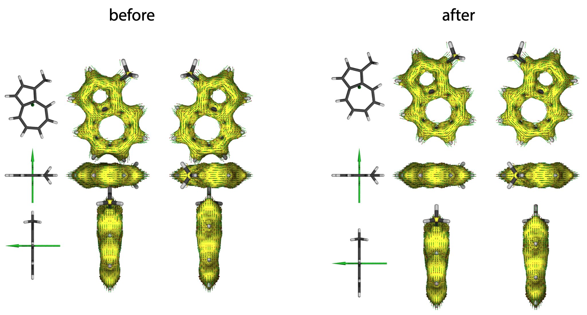
(2) Geometries are overlapping with others
If the molecule is overlapping to each other, please modify the object translate coordinates in the end of the file. The value also consists with <x, y, z> coordinates, z should always be 0 (on the plane).
object           // vertical view in the 1st column
{ MolUndMag
  translate < -45,32,0 >
}
object           // front view in the 1st column
{ MolUndMag
  rotate < 90,0,0 >
  translate < -45,0,0 >
}
object           // side view in the 1st column
{ MolUndMag
  rotate < 0,90,0 >
  translate < -45,-32,0 >
}


object           // vertical view in the 2nd column
{ MolUndIso
  translate < -10,29,0 >
}
object           // front view in the 2nd column
{ MolUndIso
  rotate < 90,0,0 >
  translate < -10,0,0 >
}
object           // side view in the 2nd column
{ MolUndIso
  rotate < 0,90,0 >
  translate < -10,-29,0 >
}

object           // vertical view in the 3rd column
{ MolUndIso
  rotate < 0,180,0 >
  translate < 35,29,0 >
}
object           // front view in the 3rd column
{ MolUndIso
  rotate < 90,0,0 >
  rotate < 0,180,0 >
  translate < 35,0,0 >
}
object           // side view in the 3rd column
{ MolUndIso
  rotate < 0,90,0 >
  rotate < 0,180,0 >
  translate < 35,-29,0 >
}
Enjoy Reading This Article?
Here are some more articles you might like to read next: